Slope and altitude based materials in Cycles

If you've used any graphics program that specializes in landscape generation, such as Terragen, you have probably seen that a core feature is the ability to automatically calculate the borders between snow, barren stone and grass from the geometry. Snow is only possible above a certain altitude where the temperature is below the freezing point, and even there snow will not stick on surfaces that slope too steeply. Similarly, grass will only be found below a certain altitude where it's warm enough, and will also not grow on too steeply sloping ground.

Previous proposed solutions use light groups, but I find these a bit unintuitive and unwieldy, so I use a more direct method by using the normal vectors to choose the material.

A suitable mountain terrain can be generated using the ANT Landscape add-on. There are numerous tutorials on using this add-on, so I will just provide a .blend file with a pregenerated terrain, as well as simple premade rock and snow materials.

Using slope to choose texture

We'll start by showing the basic principle, which only requires a few nodes. First, select the Landscape mesh object and create a new material by pressing the New button in the Material tab. Rename it to Terrain. A Diffuse BSDF with a white color will be added by default. Create a duplicate of the Diffuse BSDF by selecting it, hitting shift + D, and dragging and dropping it below the original copy. Change the color of the duplicate to any color that contrasts well with white, such as deep blue. To mix both colors, press shift + A and add a Shader→Mix Shader. Connect the BSDF outputs from the Diffuse BSDF nodes to the Shader inputs of the Mix Shader, and connect its Shader output to the Surface port of the Material Output node.

We now want one of these two colors to be used at each point of the mesh depending on the inclination at that point. To get access to information on the geometry of the object, press shift + A to add a new node and choose Input→Geometry. Mathematically, we want to look at the direction of the normal vector of the mesh. A normal vector $\mathbf{\hat{n}}$ is a vector pointing straight out from a surface to the direction that the surface is facing, as illustrated in Figure 1. We are interested in the angle between this normal vector and a fixed vector pointing straight upwards, which we call $\mathbf{\hat{z}}$, as shown in Figure 2.

From linear algebra, we know that $$ \mathbf{\hat{n}} \cdot \mathbf{\hat{z}} = \cos \theta $$ where $\theta$ is the desired angle, and the dot denotes the dot product. Solving for the angle gives $$ \theta = \arccos (\mathbf{\hat{n}} \cdot \mathbf{\hat{z}}) $$ So, add a Converter→Vector Math node and change the vector operation from the default Add to Dot Product in the drop-down list inside the node. To plug in the normal vector $\mathbf{\hat{n}}$, connect the True Normal output from the Geometry node to the first Vector input. The difference between the Normal and True Normal ports will be explained later in this tutorial when the distinction becomes important. For the other Vector input, click on the drop-down list for this port and manually enter the three numbers $(0, 0, 1)$. These are just the x, y and z components of the fixed $\mathbf{\hat{z}}$ unit vector. Next, add a Converter→Math node and change its operation to Arccosine. Connect the gray Value output of the Dot Product to the first Value input of the Arccosine node.

We have now produced the angle $\theta$. To choose color based on this angle, add another Math node and change its operation to Greater than. Connect the output from the Arccosine node to the first input of the Greater than node, and connect its output to the Fac input of the Mix Shader. The desired threshold angle could now be typed in directly at the second input of the Greater than node, but we would have to specify it in radians. To be able to use degrees instead, add another Math node and make it a Multiply node. Connect its output to the Greater than node, then click on its second input port and type pi/180, the conversion factor from degrees to radians. Note how the value of $\pi / 180$ is evaluated automatically by Blender. Now the first input of this node can be fed with the threshold angle in degrees. 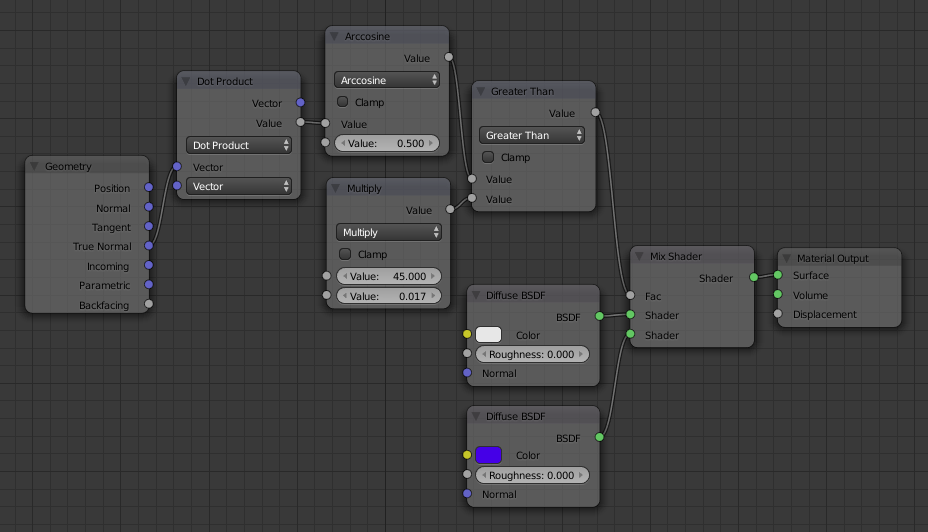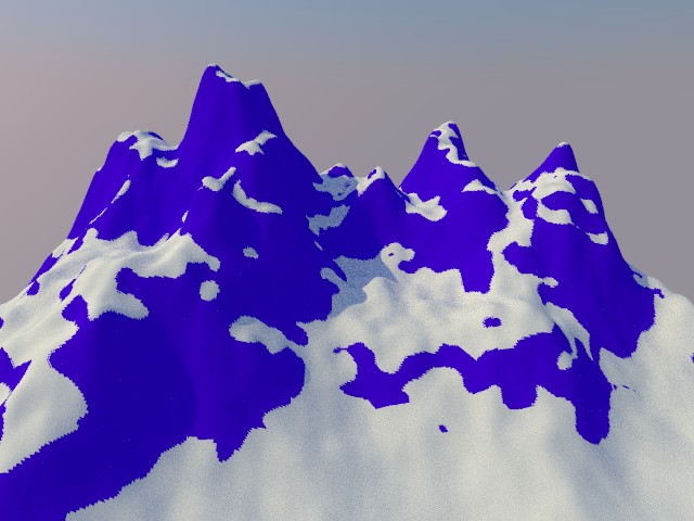Enter 45 for a first test, and change Viewport Shading of the 3D View window to Rendered to see the result. Figure 3 shows the full node setup at this point, and Figure 4 shows the result. All parts of the mountain with an inclination of 45° or less is white, and the rest is blue.

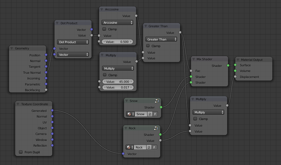
Now that we have seen the working principle, let's switch to the premade rock and snow materials in order to get something that actually looks like a snow-covered mountain. Delete the two Diffuse BSDFs and add a Group→Snow to replace the white one and a Group→Rock to replace the blue one (connecting their outputs to the Mix Shader). Next, add a Input→TextureCoordinate and connect its Generated output to the Vector input of the Rock node.

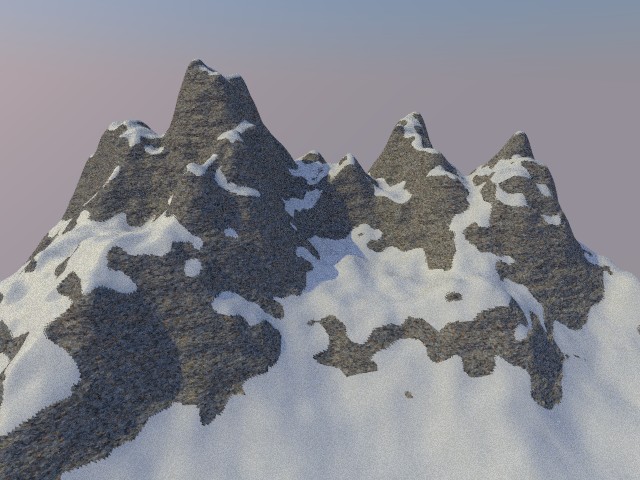
The mountain may now have a rock texture, but looks quite plastic as you can see. This is because there is no displacement map in place, so that the surface is completely smooth. The Rock material group provides a displacement output, but if you connect it directly to the Displacement port of the Material Output node (try it!), it will affect all of the mountain, even where the snow is. We already have a Greater Than node in place that “selects” the parts that are not covered by snow. What we need to do is to multiply the displacement value with the output of the Greater Than node by adding a Math node. Figure 5 shows what the node setup should now look like, and Figure 6 shows a render at this point. At this point it becomes important that we used the True Normal output from the Geometry. The True Normal port gives the normal of the raw mesh, while the Normal port includes displacement maps and mesh smoothing. In this case, we are using the normal vector port to calculate the displacement map, so using the True Normal would create an infinite loop: The True Normal would determine the displacement, but the displacement would be included in the True Normal. I don't know how Blender breaks free from such an infinite loop, I can tell that it doesn't hang or crash, but the result wasn't good.

Smoothing the snow lines

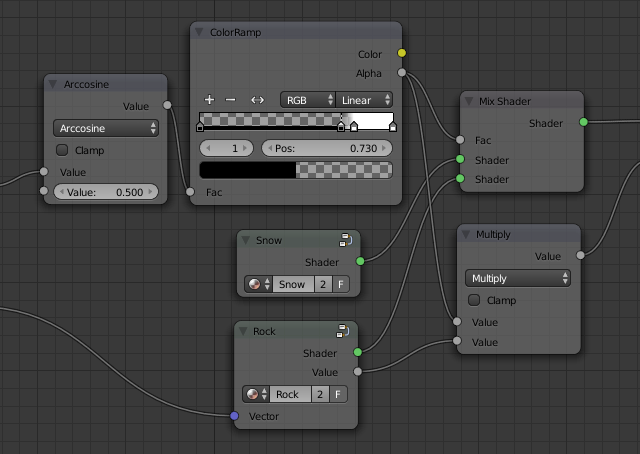
The border between rock and snow now looks very sharp and pixelated, so let's make it a bit smoother. The border is sharp because the Greater Than node only outputs two values, 0 (giving all snow) and 1 (giving no snow). The most common way got get a softer transition is to use a ColorRamp node with two color stops close to each other, as shown in Figure 7. But even though such a color ramp only takes a minute or two to setup, I find that I want this effect so often that I have instead created a reusable node group, composed of math nodes, for this purpose. This also has the advantage that the threshold value and the smoothness can be controlled by a variable from another node if desired (though we won't do that in this tutorial). If you hate math and love playing around with color ramps, you may skip this section and do as shown in Figure 7 instead.

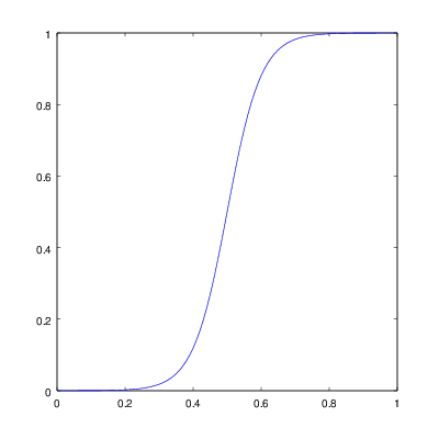
We need a function that stays at zero for some time, then gently climbs up to one and again stays there. There are a number of such S-shaped mathematical functions, but I have chosen the logistic function for its simplicity. It is given by $$ f(x) = { 1 \over {1 + e^{s(m-x)}} } $$ and is plotted in Figure 8. The constant $s$ controls sharpness of the transition (lower values make it more smooth) and $m$ contains the threshold value. So how do we translate this formula to Blender math nodes? The key is to think about what operations are involved in the formula and in what order they need to be performed. The part within parentheses in a mathematical formula are always evaluated before the part outside those parentheses, so we have to start with the $m-x$ part by using a Subtract node (all math nodes are created by adding a Converter→Math node and then choosing an operation in the drop-down list). The result needs to be multiplied by $s$ using a Multiply node. I haven't told you where to get the constant values from yet, leave them unconnected and we will return to them in a minute. For the “$e$ to the power of” part, use a Power node, click on its first input, and just type e (Blender will again substitute the value of Euler's number). Next use an Add node and finally a Divide node. For the details of all connections, refer to Figure 9.

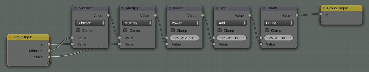
Now select all those math nodes and click on Node→Make Group or just press ctrl + G. Now that we have created a group, the function argument $x$ and the $s$ and $m$ constants can be made inputs of that group by connecting each of them to the automatically created Group Input node. Similarly, the final output from the Divide node should be connected to the Group Output node. Create new connections to these special input/output nodes by dragging from the empty circle to another node port. The inputs and outputs now also appears in the list called Interface in the GUI. Click on each one of them and give them a name, a default value, a minimum value and a maximum value. I'd like to call the function argument x and give it a default value of 0 (leave the min and max values as is). The $m$ constant can be named Midpoint and have a default value of 0.5, a minimum value of 0 and a maximum value of 1. The $s$ constant can be named Scale and have a default value of 50, a minimum value of 1, and a maximum value of 100. The output can be named y and its other values left as is (I don't think they are used for outputs). The node setup should now look exactly as in Figure 9. Finally, press shift + tab to exit the group, and with the group still selected change its name under Properties to Logistic function.

The node group that we just created can be reused in other .blend files by using the File→Link or File→Append commands. For now, let's replace the Greater Than node with our new Logistic function node. The output from the Arccosine node should be connected to the x input port, the output from the Multiply node should be connected to the Midpoint input port, and the Scale input can be set to a constant value of 30. The y output should replace the connections from the Greater Than node to both the Mix Shader and the Multiply nodes. The snow border should now look smoother and more natural than before. You can play with the Scale value to very easily change the smoothness.

Using altitude as well

Let's move on to limit the snow to only cover the mountain above the snow line. The principle is the same, but now we use the Position output from the Geometry node. Here too we are only interested in the z component of the position vector since this represents the altitude, so create a copy of the Dot Product node by selecting it and hitting shift + D, and connect the Position vector to its first input. Also create a copy of the Logistic function and connect the Value (gray) output of the Dot Product to the x input of the Logistic function. Now connect the output of the Logistic function to the Mix Shader node, replacing the previous connection. We got the opposite of what we wanted - only the bottom part of the mountain is covered by snow, so we must invert the signal. Insert a Subtract math node, set its first input to a constant 1, and connect the new Logistic function to its second input. Connect its output to both the Mix Shader and the Multiply node for the displacement.

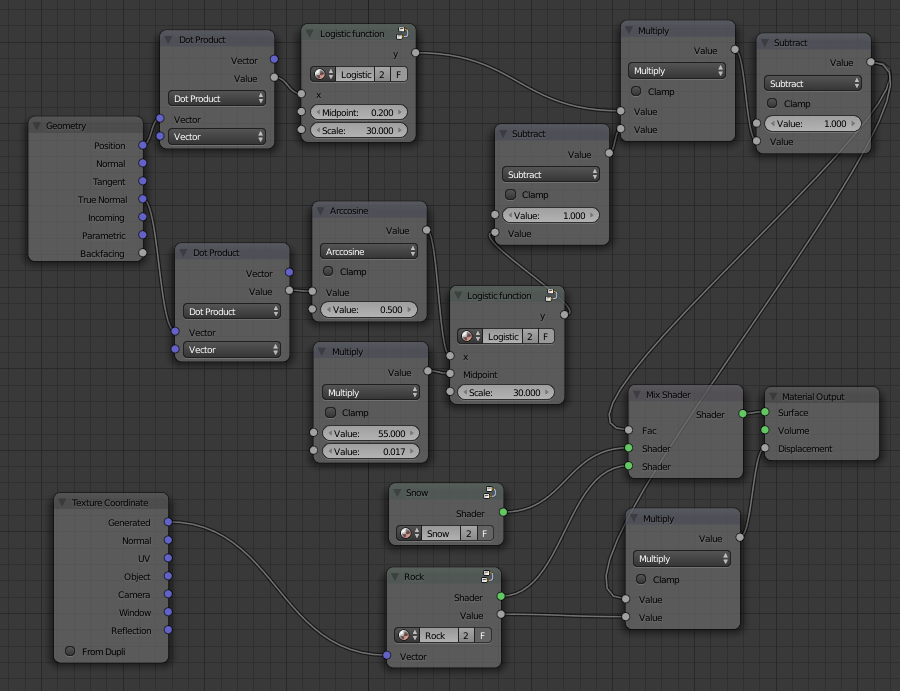
The top part of the mountain should now be completely covered by snow. We still don't want the steep slopes to be covered, so we now need to combine the two conditions. If snow was always represented by 1 and bare rock was always represented by 0 it would just be a matter of multiplying the two signals. However, most of the signals work the other way around. Delete the Subtract node we just added and add a new one to instead invert the output from the old Logistic function. Combine the two signals using a new Multiply node, invert its output with another Subtract node, and connect the final output to the Mix Shader and the displacement Multiply node. The nodes should now look as in Figure 10.

A finishing touch

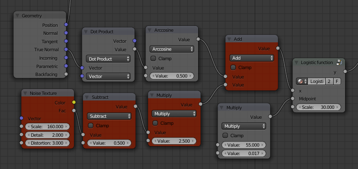
The spots of snow are now very big, which looks unrealistic. This is due to the limited resolution of the mesh. We can easily cheat and simulate a more detailed mesh by adding a random component to the snow line. Figure 11 shows the new nodes needed colored in red. The Noise Texture node simulates the detailed variations in slope of the mountain. Since it will provide only positive values between 0 and 1, it would only increase the slope, so we subtract 0.5 to have it both increase and decrease it. We then multiply it by 2.5 to fine tune the impact of this new random component, and finally add it to the slope value that we had before. Figure 12 shows the rendered scene after this last modification.

We are not aiming for photo realism here, but I hope to have provided some insights in getting the node editor to select materials based on your desired conditions, and that I managed to explain some of the mathematics inherent in the node editor. It is often possible to accomplish the wanted results without understanding the math, but getting this understanding can be helpful and satisfying nevertheless.